Introduction to combinatorial demultiplexing

Jakob Peder Pettersen

UiT, the Arctic University of Norway, Department of Computer Science
jakobpeder.pettersen@gmail.com

21 January 2026

Basics

When and why to use this package

This package is aimed at single-cell RNA-seq approaches such as SPLiT-seq [1; 2], BacDrop [3], and PETRI-seq [4; 5]. Here, each cell to be sequenced is defined by its own unique combination of multiple DNA barcodes. We do assume that the individual barcodes come from a predefined whitelist, but that the combination of barcodes is random and that every possible combination of barcodes is valid. In order to identify from which cell each read is coming from, we must extract the barcodes, compare them with the reference barcodes, and find the best match.

Required knowledge

posDemux uses the Biostrings package for handling sequencing data and hence a basic understanding of Biostrings is necessary to use this package. Also important to note is the fact that while posDemux does provide utilities for demultiplexing scRNA-seq data, it is designed to be part of a greater workflow. In particular, the package does not include essential components of a scRNA-seq workflow like quality control, alignment, feature counting and UMI deduplication, neither does it provide any utilities for tertiary analysis once the gene count matrix is constructed. Hence, the user should be familiar with the other components of such workflows [2] and know how the functionality of this package plays a part therein.

If you are asking yourself the question “Where do I start using Bioconductor?” you might be interested in this blog post.

Limitations

Since this is a positional demultiplexer, the position of all segments and barcodes must be known in advance and be the same for all reads. Hence, the package is not suited in cases where segments occur at variable positions among the reads. Furthermore, in the cases where the segments are at fixed positions among the reads, but the segment lengths are unknown, it may require some trial and error to obtain the correct segmentation.

The demultiplexer is written with Illumina sequencing in mind. It assumes that substitution sequencing errors may occur, but has no safeguard against indel sequencing errors. Hence, indel errors will result in erroneous segmentation and failure to assign the correct barcode. For sequencing platforms where indel errors are common, such as Nanopore sequencing, this package may therefore not be suitable.

This package does not by itself support combining barcodes on both reverse and forward reads, but this limitation can be circumvented by either artificially merging reads or manipulating the result structures from the demultiplexer.

Ways to interact with this package

This vignette describes the basic usage of the package where the FASTQ files are read into R before the demultiplexing begins. For large datasets or memory-limited systems, reading all sequences into memory at once is too taxing. For this reason, posDemux has a streaming API where only parts of the input file is read at a time. For brevity, this functionality is explained in its own vignette (vignette("streaming")). We believe that most end-users won’t interact with this package directly, but rather in the form of a custom-made bioinformatic pipeline. Also, we think that most developers of bioinformatics pipelines would prefer the streaming API. Still, we think those developing with this package should have an understanding of its low-level API as to understand what it does under the hood.

Install posDemux

This package is hosted on Bioconductor repository for R packages. In order to install it from a fresh R install, run:

if (!requireNamespace("BiocManager", quietly = TRUE)) {
    install.packages("BiocManager")
}

BiocManager::install("posDemux")

## Check that you have a valid Bioconductor installation
BiocManager::valid()

If you want to obtain the development version of the package, it is available on GitHub:

if (!requireNamespace("devtools", quietly = TRUE)) {
    install.packages("devtools")
}

devtools::install("yaccos/posDemux")

If you compile the package from source, we do recommend you use the compiler flag -ftree-vectorize as this provides considerable speedup to the demultiplexer.

Asking for help

As package developers, we try to explain clearly how to use our packages and in which order to use the functions. But R and Bioconductor have a steep learning curve so it is critical to learn where to ask for help. The blog post quoted above mentions some but we would like to highlight the Bioconductor support site as the main resource for getting help: Remember to use the posDemux tag and check the older posts. Other alternatives are available such as creating GitHub issues and tweeting. However, please note that if you want to receive help you should adhere to the posting guidelines. It is particularly critical that you provide a small reproducible example and your session information so package developers can track down the source of the error.

Citing posDemux

We hope that posDemux will be useful for your research. Please use the following information to cite the package and the overall approach. Thank you!

## Citation info
citation("posDemux")
#> To cite package 'posDemux' in publications use:
#> 
#>   Pettersen J (2025). _posDemux: Positional combinatorial sequence
#>   demultiplexer_. R package version 0.99.10,
#>   <https://github.com/yaccos/posDemux>.
#> 
#> A BibTeX entry for LaTeX users is
#> 
#>   @Manual{,
#>     title = {posDemux: Positional combinatorial sequence demultiplexer},
#>     author = {Jakob Peder Pettersen},
#>     year = {2025},
#>     note = {R package version 0.99.10},
#>     url = {https://github.com/yaccos/posDemux},
#>   }

An example with PETRI-seq

Quick overview of the method

The PETRI-seq method is a method for single-cell RNA-sequencing of bacteria [4; 5]. It uses paired-end Illumina sequencing where the forward read contains the cell barcodes and the transcript UMI, whereas the reverse read contain the cDNA to be aligned to the genome. Hence, posDemux will only be applied to the forward reads. We start by loading the posDemux itself and some helper packages:

library(posDemux)
library(Biostrings)
library(purrr)
library(magrittr)

Sequence annotation

For PETRI-seq, the forward read consists of the following segments in the following order (from 5’ to 3’):

• UMI: 7 nucletides
• Barcode 3(bc3) : 7 nucleotides
• Linker: 15 nucletides
• Barcode 2(bc2): 7 nucleotides
• Linker: 14 nucletides
• Barcode 1(bc1): 7 nucleotides
• The rest of the read is ignored

Hence, we consider the first segment, the UMI, as a payload (denoted as P in the sequence annotation) to be kept. The three barcodes (denoted as B) are used for demultiplexing. Finally, the linkers and the read past Barcode 1 (denoted as A) are ignored.

We specify it with as:

sequence_annotation <- c(UMI = "P", "B", "A", "B", "A", "B", "A")
segment_lengths <- c(7L, 7L, 15L, 7L, 14L, 7L, NA_integer_)

Data loading

For the demultiplexing, we need the listing of the barcodes, and of course the reads to demultiplex. For this package, the PETRI-seq barcodes and synthetically generated reads are provided. We load the barcodes:

barcode_files <- system.file("extdata/PETRI-seq_barcodes",
    c(
        bc1 = "bc1.fa",
        bc2 = "bc2.fa",
        bc3 = "bc3.fa"
    ),
    package = "posDemux"
)
names(barcode_files) <- paste0("bc", 1L:3L)
barcode_index <- map(barcode_files, readDNAStringSet)

… and the FASTQ file containing the forward reads:

input_fastq <- system.file("extdata",
    "PETRI-seq_forward_reads.fq.gz",
    package = "posDemux"
)
reads <- readDNAStringSet(input_fastq, format = "fastq")

posDemux accepts both DNAStringSet and QualityScaledDNAStringSet as input where the latter contain the quality scores of the reads. However, the quality score is ignored by the demultiplexer and the only reason to pass a QualityScaledDNAStringSet is when it is desirable to retain the quality scores in the payload.

Running the demultiplexer

Before we run the demultiplexer, we must ensure that the barcodes index is arranged in the correct order:

barcodes <- barcode_index[c("bc3", "bc2", "bc1")]

We are now ready to run the demultiplexer:

demultiplex_res <- combinatorial_demultiplex(
    reads,
    barcodes = barcodes,
    segments = sequence_annotation,
    segment_lengths = segment_lengths
)

The main results from this demultiplexer are the table of assigned barcodes:

head(demultiplex_res$assigned_barcodes)
#>       bc3      bc2      bc1     
#> seq_1 "bc3_57" "bc2_51" "bc1_94"
#> seq_2 "bc3_72" "bc2_94" "bc1_95"
#> seq_3 "bc3_23" "bc2_37" "bc1_85"
#> seq_4 "bc3_85" "bc2_81" "bc1_17"
#> seq_5 "bc3_49" "bc2_64" "bc1_77"
#> seq_6 "bc3_3"  "bc2_45" "bc1_33"

the table of mismatches to the barcode:

head(demultiplex_res$mismatches)
#>       bc3 bc2 bc1
#> seq_1   0   0   0
#> seq_2   0   0   0
#> seq_3   2   2   2
#> seq_4   0   0   0
#> seq_5   0   0   0
#> seq_6   0   0   0

as well as the extracted UMI sequences:

demultiplex_res$payload$UMI
#> DNAStringSet object of length 56895:
#>         width seq                                           names               
#>     [1]     7 GCCTAAC                                       seq_1
#>     [2]     7 CCAAGCG                                       seq_2
#>     [3]     7 AGTGCAC                                       seq_3
#>     [4]     7 CCTAACG                                       seq_4
#>     [5]     7 GCTCGTC                                       seq_5
#>     ...   ... ...
#> [56891]     7 ACGGCTT                                       seq_56891
#> [56892]     7 ATGAGCG                                       seq_56892
#> [56893]     7 ACCTGCG                                       seq_56893
#> [56894]     7 GGATATC                                       seq_56894
#> [56895]     7 GCCTTGA                                       seq_56895

Error correction

posDemux handles two types reads filtering:

• Retaining only the reads being matched with a barcode combination after error correction.
• Removing barcode combinations which have few reads as these are usually artifacts and are not assumed to cover the transcripts of an entire cell.

This subsection consider the first type of filtering. During demultiplexing,the barcode with the smallest Hamming distance to the read is chosen and the number of mismatches is recorded. If there are multiple barcodes being equal in distance to the query, one of these barcodes is chosen. When there are no mismatches for any of the barcode sets, we obviously want to keep this read. When one or more barcode has mismatches, posDemux allows for error correction. In that case, we will keep the read if the number of mismatches to each of its barcodes is below a certain threshold.

In our example, the smallest Hamming distance between two different barcodes is $3$ for all barcode sets. Given $n$, the number of barcode sequencing errors which can be reliably corrected in a barcode set, the minimum distance required between two distinct barcodes needs to be at least $2n+1$. This means that in our case, we can correct for exactly one sequencing error:

filtered_res <- filter_demultiplex_res(
    demultiplex_res,
    allowed_mismatches = 1L
)

We will now inspect the summary of the demultiplexing and filtering:

filtered_res$summary_res
#> Total number of reads: 56895 
#> Number of reads failing to demultiplex: 4989 (8.77%) 
#> Observed number of unique barcode combinations:978 
#> Number of possible barcode combinations: 884736 
#> Estimated number of features: 978.5 
#> Observed feature to barcode ratio: 0.001105 
#> Corrected feature to barcode ratio: 0.001106 
#> Estimated number of observed barcode combinations
#> corresponding to more than one feature: 0.5 (0.06%) 
#> Number of barcode sets: 3 
#> - - - - - - - - - - - - - - - - - - - - - - - - - - - - - - - - - - - - - - - - - - - - - - - - - - - - - - - - - - - - - - - - - - - - - - - - - - - - - - - - 
#> Barcode set: bc3 
#> Barcode width: 7 
#> Number of possible barcodes: 96 
#> Number of allowed mismatches: 1 
#> Number of reads with 0 mismatches: 51923 (91.26%) 
#> Number of reads with 1 mismatches: 671 (1.18%) 
#> Number of reads above mismatch threshold: 4301 (7.56%) 
#> - - - - - - - - - - - - - - - - - - - - - - - - - - - - - - - - - - - - - - - - - - - - - - - - - - - - - - - - - - - - - - - - - - - - - - - - - - - - - - - - 
#> Barcode set: bc2 
#> Barcode width: 7 
#> Number of possible barcodes: 96 
#> Number of allowed mismatches: 1 
#> Number of reads with 0 mismatches: 51918 (91.25%) 
#> Number of reads with 1 mismatches: 567 (1%) 
#> Number of reads above mismatch threshold: 4410 (7.75%) 
#> - - - - - - - - - - - - - - - - - - - - - - - - - - - - - - - - - - - - - - - - - - - - - - - - - - - - - - - - - - - - - - - - - - - - - - - - - - - - - - - - 
#> Barcode set: bc1 
#> Barcode width: 7 
#> Number of possible barcodes: 96 
#> Number of allowed mismatches: 1 
#> Number of reads with 0 mismatches: 51930 (91.27%) 
#> Number of reads with 1 mismatches: 642 (1.13%) 
#> Number of reads above mismatch threshold: 4323 (7.6%) 
#> - - - - - - - - - - - - - - - - - - - - - - - - - - - - - - - - - - - - - - - - - - - - - - - - - - - - - - - - - - - - - - - - - - - - - - - - - - - - - - - -

Now, the results in filtered_res$demultiplex_res only shows the reads either without mismatches or where error correction could be applied:

head(filtered_res$demultiplex_res$assigned_barcodes)
#>       bc3      bc2      bc1     
#> seq_1 "bc3_57" "bc2_51" "bc1_94"
#> seq_2 "bc3_72" "bc2_94" "bc1_95"
#> seq_4 "bc3_85" "bc2_81" "bc1_17"
#> seq_5 "bc3_49" "bc2_64" "bc1_77"
#> seq_6 "bc3_3"  "bc2_45" "bc1_33"
#> seq_7 "bc3_17" "bc2_57" "bc1_71"
head(filtered_res$demultiplex_res$mismatches)
#>       bc3 bc2 bc1
#> seq_1   0   0   0
#> seq_2   0   0   0
#> seq_4   0   0   0
#> seq_5   0   0   0
#> seq_6   0   0   0
#> seq_7   0   0   0

We can also see which reads are retained:

head(filtered_res$retained)
#> seq_1 seq_2 seq_3 seq_4 seq_5 seq_6 
#>  TRUE  TRUE FALSE  TRUE  TRUE  TRUE

Filtering by barcode frequency

Now as we have conducted the filtering based on barcode mismatches, we proceed with the second kind of filtering. It utilizes the Knee method [6; 4] where the barcode combinations are arranged in descending order on frequency and the most abundant ones are selected. The cutoff is set such that we achieve a saturation where most reads are covered, yet the remaining barcode combinations not covered all have a small number of reads.

We first create a frequency table of the barcodes is question:

freq_table <- create_freq_table(
    filtered_res$demultiplex_res$assigned_barcodes
)
head(freq_table)
#>      bc3    bc2    bc1 frequency cumulative_frequency    fraction
#> 1 bc3_37  bc2_4 bc1_30       270                  270 0.005201711
#> 2 bc3_45 bc2_36 bc1_65       246                  516 0.004739336
#> 3 bc3_25 bc2_34 bc1_25       235                  751 0.004527415
#> 4 bc3_40 bc2_62 bc1_42       221                  972 0.004257697
#> 5 bc3_69 bc2_95 bc1_37       219                 1191 0.004219165
#> 6 bc3_29 bc2_90 bc1_40       217                 1408 0.004180634
#>   cumulative_fraction
#> 1         0.005201711
#> 2         0.009941047
#> 3         0.014468462
#> 4         0.018726159
#> 5         0.022945324
#> 6         0.027125958

This package contains an interaction Shiny application for selecting the number of barcodes. It can be run by:

interactive_bc_cutoff(freq_table)

If you are working outside RStudio, you may have to run

app <- interactive_bc_cutoff(freq_table)
shiny::runApp(app, launch.browser = FALSE)

and opening the resulting link inside the browser. If you are working on a headless system, you may consider:

• Using RStudio Server
• Opening a reverse ssh tunnel for the Shiny server
• Copy the frequency table onto your local machine and run the application there

If you run the application, you will see that keeping approximately 500 barcodes is the optimal choice¹. We can also calculate the frequency of the least abundant barcode combination being included.

bc_cutoff <- 500L
freq_cutoff <- bc_to_freq_cutoff(freq_table, bc_cutoff)
freq_cutoff
#> [1] 8

We can convert the cutoff the other way as well, but it is in general not an exact inverse as multiple barcodes can have the same frequency:

reconstrued_bc_cutoff <- freq_to_bc_cutoff(
    freq_table,
    freq_cutoff
)
reconstrued_bc_cutoff
#> [1] 505

The cutoff can be illustrated by the Knee plot as in the interactive application:

knee_plot(freq_table = freq_table, cutoff = bc_cutoff)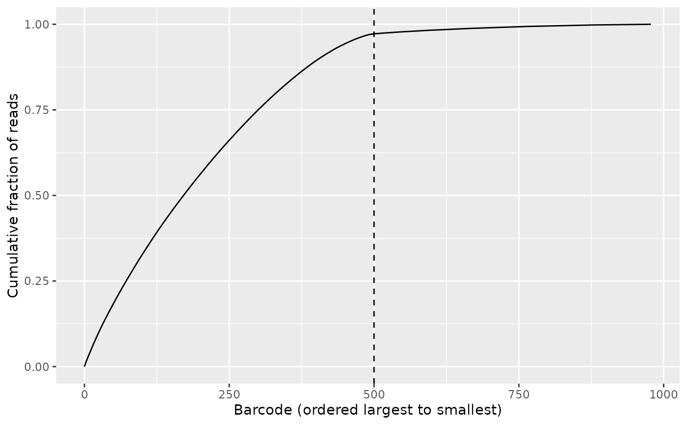

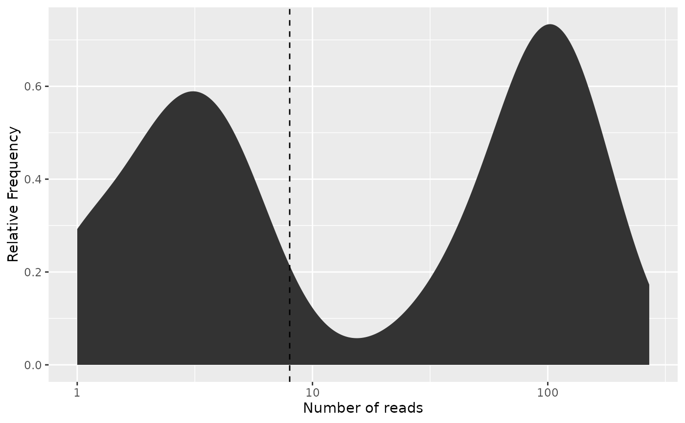
We can also illustrate this filtering by looking at the distribution of barcode frequencies:

# Since the cutoff lines of the plot are provided by the literal x-coordinate,
# we must use the frequency cutoff
freq_plot(freq_table,
    cutoff = freq_cutoff, type = "density",
    log_scale_x = TRUE
)

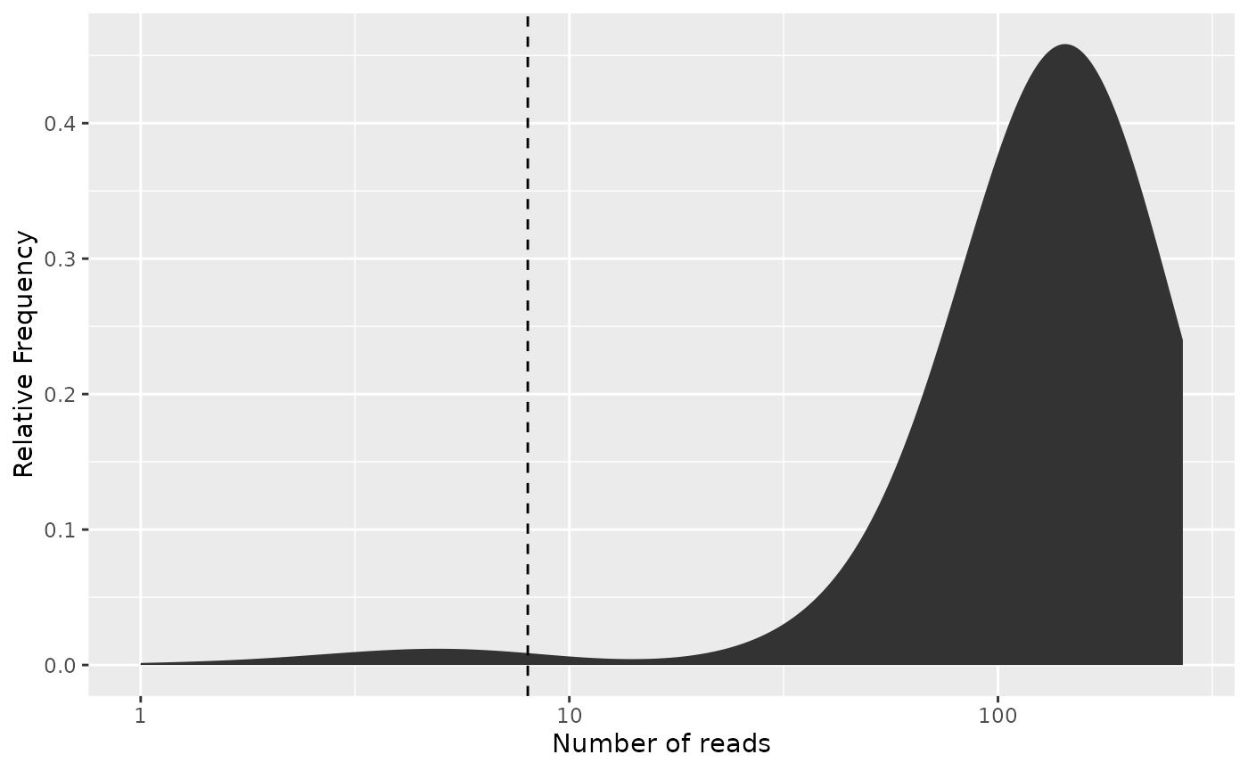
Often the frequency plot gets easier to interpret when we scale the y-axis by the number of reads, hence creating a mass plot of where the reads are distributed based on their respective barcodes:

# Since the cutoff lines of the plot are provided by the literal x-coordinate,
# we must use the frequency cutoff
freq_plot(freq_table,
    cutoff = freq_cutoff, type = "density",
    log_scale_x = TRUE, scale_by_reads = TRUE
)

Exporting results

Now as we know how many barcodes to keep, we can extract the desired results and write it to a table.

We start with the frequency table. Since it is already sorted in descending order of frequency, we simply take the top entries in the table:

selected_freq_table <- freq_table[seq_len(bc_cutoff), ]

For finding which reads correspond to these barcodes, we do the following:

assigned_barcodes <- filtered_res$demultiplex_res$assigned_barcodes
read_in_selection <- row_match(assigned_barcodes, selected_freq_table)
selected_assigned_barcodes <- assigned_barcodes[read_in_selection, ]

We continue with the UMIs which we convert to a character vector (remember that the payload and assigned barcodes are aligned in order):

assigned_UMI <- filtered_res$demultiplex_res$payload$UMI %>% as.character()
selected_assigned_UMI <- assigned_UMI[read_in_selection]

With all of this done, we can make a data frame containing the UMI, read identifier, and barcode assignments:

res_table <- as.data.frame(selected_assigned_barcodes) %>%
    dplyr::mutate(
        read = rownames(selected_assigned_barcodes),
        UMI = selected_assigned_UMI
    ) %>%
    # Ensures the columns appears in the desired order
    dplyr::select(read, UMI, bc3, bc2, bc1)
head(res_table)
#>        read     UMI    bc3    bc2    bc1
#> seq_1 seq_1 GCCTAAC bc3_57 bc2_51 bc1_94
#> seq_2 seq_2 CCAAGCG bc3_72 bc2_94 bc1_95
#> seq_4 seq_4 CCTAACG bc3_85 bc2_81 bc1_17
#> seq_5 seq_5 GCTCGTC bc3_49 bc2_64 bc1_77
#> seq_6 seq_6 TGGAGAA  bc3_3 bc2_45 bc1_33
#> seq_7 seq_7 ACTTCGA bc3_17 bc2_57 bc1_71

Finally, we can write the table to file. The following is the suggested way for achieving the desired formatting:

file <- tempfile(pattern = "barcode_table", fileext = ".txt")
write.table(res_table, file,
    row.names = FALSE,
    col.names = TRUE, sep = "\t", eol = "\n", quote = FALSE
)

Reproducibility

The posDemux package
was made possible thanks to:

• R
• BiocStyle
• knitr
• RefManageR
• rmarkdown
• sessioninfo
• testthat

This package was developed using biocthis.

R session information:

#> ─ Session info ───────────────────────────────────────────────────────────────────────────────────────────────────────
#>  setting  value
#>  version  R Under development (unstable) (2026-01-20 r89309)
#>  os       Ubuntu 24.04.3 LTS
#>  system   x86_64, linux-gnu
#>  ui       X11
#>  language en
#>  collate  C.UTF-8
#>  ctype    C.UTF-8
#>  tz       UTC
#>  date     2026-01-21
#>  pandoc   3.1.11 @ /opt/hostedtoolcache/pandoc/3.1.11/x64/ (via rmarkdown)
#>  quarto   NA
#> 
#> ─ Packages ───────────────────────────────────────────────────────────────────────────────────────────────────────────
#>  package      * version date (UTC) lib source
#>  assertthat     0.2.1   2019-03-21 [1] RSPM
#>  backports      1.5.0   2024-05-23 [1] RSPM
#>  bibtex         0.5.1   2023-01-26 [1] RSPM
#>  BiocGenerics * 0.57.0  2025-10-30 [1] Bioconduc~
#>  BiocManager    1.30.27 2025-11-14 [1] RSPM
#>  BiocStyle    * 2.39.0  2025-10-30 [1] Bioconduc~
#>  Biostrings   * 2.79.4  2026-01-07 [1] Bioconduc~
#>  bookdown       0.46    2025-12-05 [1] RSPM
#>  bslib          0.9.0   2025-01-30 [1] RSPM
#>  cachem         1.1.0   2024-05-16 [1] RSPM
#>  cli            3.6.5   2025-04-23 [1] RSPM
#>  crayon         1.5.3   2024-06-20 [1] RSPM
#>  desc           1.4.3   2023-12-10 [1] RSPM
#>  digest         0.6.39  2025-11-19 [1] RSPM
#>  dplyr          1.1.4   2023-11-17 [1] RSPM
#>  evaluate       1.0.5   2025-08-27 [1] RSPM
#>  farver         2.1.2   2024-05-13 [1] RSPM
#>  fastmap        1.2.0   2024-05-15 [1] RSPM
#>  fs             1.6.6   2025-04-12 [1] RSPM
#>  generics     * 0.1.4   2025-05-09 [1] RSPM
#>  ggplot2        4.0.1   2025-11-14 [1] RSPM
#>  glue           1.8.0   2024-09-30 [1] RSPM
#>  gtable         0.3.6   2024-10-25 [1] RSPM
#>  htmltools      0.5.9   2025-12-04 [1] RSPM
#>  htmlwidgets    1.6.4   2023-12-06 [1] RSPM
#>  httpuv         1.6.16  2025-04-16 [1] RSPM
#>  httr           1.4.7   2023-08-15 [1] RSPM
#>  IRanges      * 2.45.0  2025-10-31 [1] Bioconduc~
#>  jquerylib      0.1.4   2021-04-26 [1] RSPM
#>  jsonlite       2.0.0   2025-03-27 [1] RSPM
#>  knitr          1.51    2025-12-20 [1] RSPM
#>  labeling       0.4.3   2023-08-29 [1] RSPM
#>  later          1.4.5   2026-01-08 [1] RSPM
#>  lifecycle      1.0.5   2026-01-08 [1] RSPM
#>  lubridate      1.9.4   2024-12-08 [1] RSPM
#>  magrittr     * 2.0.4   2025-09-12 [1] RSPM
#>  mime           0.13    2025-03-17 [1] RSPM
#>  otel           0.2.0   2025-08-29 [1] RSPM
#>  pillar         1.11.1  2025-09-17 [1] RSPM
#>  pkgconfig      2.0.3   2019-09-22 [1] RSPM
#>  pkgdown        2.2.0   2025-11-06 [1] RSPM
#>  plyr           1.8.9   2023-10-02 [1] RSPM
#>  posDemux     * 0.99.10 2026-01-21 [1] local
#>  promises       1.5.0   2025-11-01 [1] RSPM
#>  purrr        * 1.2.1   2026-01-09 [1] RSPM
#>  R6             2.6.1   2025-02-15 [1] RSPM
#>  ragg           1.5.0   2025-09-02 [1] RSPM
#>  RColorBrewer   1.1-3   2022-04-03 [1] RSPM
#>  Rcpp           1.1.1   2026-01-10 [1] RSPM
#>  RefManageR   * 1.4.0   2022-09-30 [1] RSPM
#>  rlang          1.1.7   2026-01-09 [1] RSPM
#>  rmarkdown      2.30    2025-09-28 [1] RSPM
#>  S4Vectors    * 0.49.0  2025-10-30 [1] Bioconduc~
#>  S7             0.2.1   2025-11-14 [1] RSPM
#>  sass           0.4.10  2025-04-11 [1] RSPM
#>  scales         1.4.0   2025-04-24 [1] RSPM
#>  Seqinfo      * 1.1.0   2025-10-31 [1] Bioconduc~
#>  sessioninfo  * 1.2.3   2025-02-05 [1] RSPM
#>  shiny          1.12.1  2025-12-09 [1] RSPM
#>  stringi        1.8.7   2025-03-27 [1] RSPM
#>  stringr        1.6.0   2025-11-04 [1] RSPM
#>  systemfonts    1.3.1   2025-10-01 [1] RSPM
#>  textshaping    1.0.4   2025-10-10 [1] RSPM
#>  tibble         3.3.1   2026-01-11 [1] RSPM
#>  tidyselect     1.2.1   2024-03-11 [1] RSPM
#>  timechange     0.3.0   2024-01-18 [1] RSPM
#>  vctrs          0.7.0   2026-01-16 [1] RSPM
#>  withr          3.0.2   2024-10-28 [1] RSPM
#>  xfun           0.56    2026-01-18 [1] RSPM
#>  xml2           1.5.2   2026-01-17 [1] RSPM
#>  xtable         1.8-4   2019-04-21 [1] RSPM
#>  XVector      * 0.51.0  2025-10-31 [1] Bioconduc~
#>  yaml           2.3.12  2025-12-10 [1] RSPM
#> 
#>  [1] /home/runner/work/_temp/Library
#>  [2] /opt/R/devel/lib/R/site-library
#>  [3] /opt/R/devel/lib/R/library
#>  * ── Packages attached to the search path.
#> 
#> ──────────────────────────────────────────────────────────────────────────────────────────────────────────────────────

Bibliography

This vignette was generated using BiocStyle with knitr and rmarkdown running behind the scenes.

Citations made with RefManageR .

[1] A. B. Rosenberg, C. M. Roco, R. A. Muscat, et al. “Single-cell profiling of the developing mouse brain and spinal cord with split-pool barcoding”. In: Science 360.6385 (Apr. 2018), pp. 176–182. DOI: 10.1126/science.aam8999. URL: https://www.science.org/doi/10.1126/science.aam8999 (visited on 01/23/2025).

[2] L. Kuijpers, B. Hornung, M. C. G. N. van den Hout - van Vroonhoven, et al. “Split Pool Ligation-based Single-cell Transcriptome sequencing (SPLiT-seq) data processing pipeline comparison”. In: BMC Genomics 25.1 (Apr. 2024), p. 361. ISSN: 1471-2164. DOI: 10.1186/s12864-024-10285-3. URL: https://doi.org/10.1186/s12864-024-10285-3 (visited on 01/08/2025).

[3] P. Ma, H. M. Amemiya, L. L. He, et al. “Bacterial droplet-based single-cell RNA-seq reveals antibiotic-associated heterogeneous cellular states”. In: Cell 186.4 (Feb. 2023), pp. 877–891.e14. ISSN: 0092-8674. DOI: 10.1016/j.cell.2023.01.002. URL: https://www.sciencedirect.com/science/article/pii/S0092867423000028 (visited on 01/31/2025).

[4] S. B. Blattman, W. Jiang, P. Oikonomou, et al. “Prokaryotic single-cell RNA sequencing by in situ combinatorial indexing”. En. In: Nature Microbiology 5.10 (Oct. 2020), pp. 1192–1201. ISSN: 2058-5276. DOI: 10.1038/s41564-020-0729-6. URL: https://www.nature.com/articles/s41564-020-0729-6 (visited on 12/12/2024).

[5] S. B. Blattman, W. Jiang, E. R. McGarrigle, et al. “Identification and genetic dissection of convergent persister cell states”. En. In: Nature 636.8042 (Dec. 2024), pp. 438–446. ISSN: 1476-4687. DOI: 10.1038/s41586-024-08124-2. URL: https://www.nature.com/articles/s41586-024-08124-2 (visited on 01/08/2025).

[6] E. Macosko, A. Basu, R. Satija, et al. “Highly Parallel Genome-wide Expression Profiling of Individual Cells Using Nanoliter Droplets”. In: Cell 161.5 (2015), pp. 1202-1214. ISSN: 0092-8674. DOI: https://doi.org/10.1016/j.cell.2015.05.002. URL: https://www.sciencedirect.com/science/article/pii/S0092867415005498.